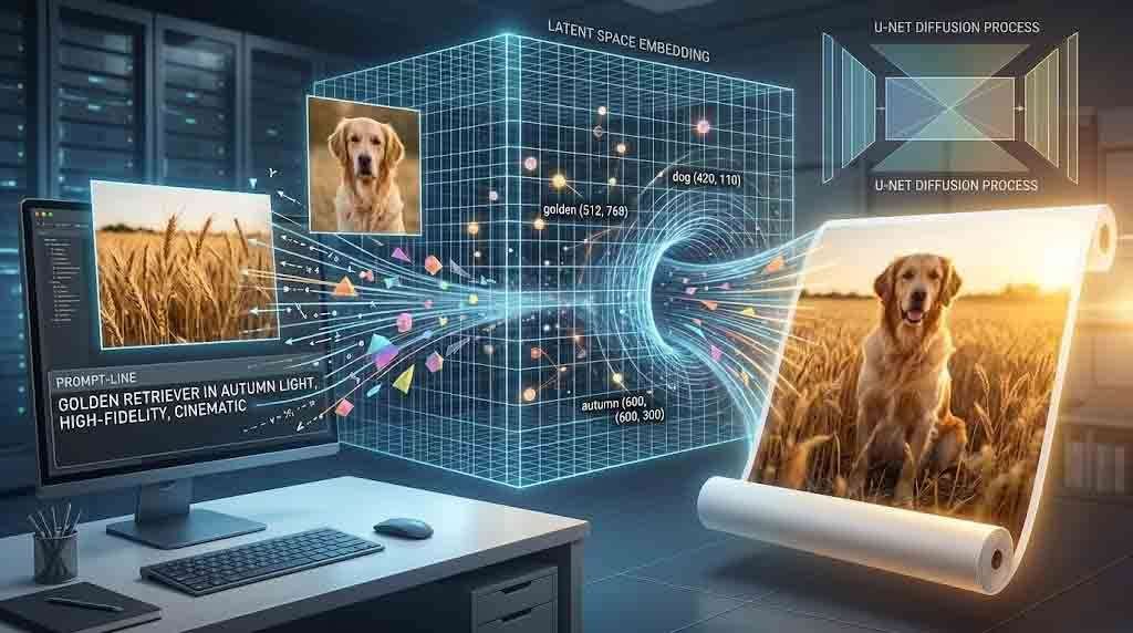
Somewhere inside a neural network, the word “golden” and a photograph of afternoon light on wheat share the same address. Not metaphorically — mathematically. They occupy nearby coordinates in a high-dimensional map that no human designed and no human fully understands, yet one that modern AI systems navigate with startling precision every time you type a prompt and watch an image materialize from noise. This is the latent space, and it is the organizing intelligence behind every text-to-image system that has reshaped creative production over the last three years.
To understand why diffusion models produce images of the quality they do — and why your word choices matter so much when prompting them — you have to follow the signal from language to pixel, step by step.
The Inefficiency of Pixel Space
An image is, at the computational level, a grid of numbers. A 512×512 RGB image contains 786,432 individual values. Training a generative model directly on that raw pixel data is possible, but profoundly expensive — the model must learn to handle nearly a million variables simultaneously for every training example, without any prior understanding of which values are meaningful and which are redundant.
Nature images, however, are not random. A face follows strict spatial logic: eyes above nose, nose above mouth. A coastline photograph has sky at the top and water at the bottom. A leather briefcase has consistent texture gradients that repeat across its surface. Natural images can be compressed into a much smaller representation without losing essential information — a principle known as the manifold hypothesis in machine learning. The high dimensionality of the raw pixel grid is, in a sense, artificial. Most of that space is empty.
Latent diffusion models exploit this fact ruthlessly. Rather than working in pixel space, they first compress the image into a latent space using a variational autoencoder (VAE) — a neural network with an encoder that converts the image to a lower-dimensional representation, and a decoder that reconstructs the image from that representation. The latent space of Stable Diffusion is 4×64×64 — 48 times smaller than the image pixel space — so the model crunches far fewer numbers at every step. The diffusion process, the most computationally intensive part of image generation, happens entirely within this compressed territory.
Forward and Reverse Diffusion: The Logic of Controlled Destruction
The diffusion framework is built on a counterintuitive premise: the best way to teach a model to create images is to first teach it to destroy them.
During training, the model takes real images from its dataset — billions of photographs, illustrations, and artworks scraped from the internet — compresses them into latent representations via the VAE encoder, and then systematically corrupts those representations by adding Gaussian noise across hundreds of steps. At each step, the image becomes slightly more degraded until, at the final timestep, nothing remains but pure statistical noise. The model observes this entire forward process — corruption from order to chaos — and learns to run it in reverse.
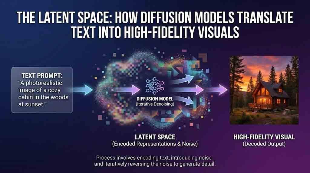
Diffusion models generate images by starting with a pattern of random noise and gradually shaping it into a coherent image through a process that reversibly adds and removes noise. At inference time — when you submit your prompt — the model starts with a randomly sampled latent noise tensor and applies its learned reverse-diffusion process: predict the noise present at the current step, subtract it, and move one increment closer to a coherent image. Repeat this for 20 to 50 steps and decode the final latent back to pixel space via the VAE decoder. What emerges is an image.
The architectural component responsible for the noise prediction at each step is the U-Net: a convolutional neural network with a characteristic hourglass shape that compresses spatial information down and then expands it back, preserving fine-grained detail through skip connections between encoder and decoder layers. The U-Net is the operational heart of the diffusion process, and it is where the text conditioning enters the picture.
How Language Becomes Geometry: CLIP and the Shared Embedding Space
The translation of a text prompt into visual output is not a simple lookup. It requires a model that has learned, across hundreds of millions of examples, that the word “baroque” and photographs of gilded ceilings and dramatic chiaroscuro belong near each other in the same mathematical space.
CLIP (Contrastive Language-Image Pre-Training) is a neural network developed by OpenAI in 2021 that jointly trains an image encoder and a text encoder to produce a shared embedding space for images and text. The training objective was elegant: given a batch of 400 million image-text pairs scraped from the internet, maximize the similarity between matching pairs and minimize the similarity between mismatched pairs. After training, the model achieves this by bringing images and their corresponding texts closer together in an embedding space while pushing apart unrelated image-text pairs.
The practical consequence is that CLIP does not merely recognize that “a dog” and an image of a dog are related. It encodes relational geometry. “A running dog” sits in a different coordinate cluster than “a sleeping dog.” “A golden retriever in autumn light” occupies a specific neighborhood that combines concepts of breed, season, and photographic quality. Text-to-image models use a pretrained language or vision-language model to convert the input prompt into a text embedding, and then use a diffusion-based generative image model to produce images conditioned on that embedding.
In practice, when you type a prompt into Midjourney, Stable Diffusion, or Gemini’s image generation, your words pass through a text encoder — often CLIP’s transformer-based model — and emerge as a vector of 512 or 768 floating-point numbers. That vector is what actually guides the denoising process. The U-Net at each diffusion step uses cross-attention mechanisms to consult the text embedding, asking: given where I am in latent space right now and what this prompt is requesting, which direction should I step to reduce noise while moving toward an image that matches this description?
Classifier-Free Guidance: Turning Up the Signal
Understanding latent space also illuminates why certain prompting techniques work. One of the most important mechanisms in modern diffusion models is classifier-free guidance (CFG), a training and inference trick that dramatically sharpens the relationship between prompt and output.
During training, the model learns to generate images both with and without text conditioning — it sees the same images sometimes with their captions attached and sometimes without, as if the caption were blank. This teaches the model two distinct behaviors: unconditional generation (produce any plausible image) and conditional generation (produce an image that matches this specific text).
At inference time, both behaviors run simultaneously. The model computes the noise prediction under the unconditional case and the noise prediction under the conditional case, then extrapolates in the direction of the conditional signal by a factor controlled by the CFG scale parameter. A CFG scale of 1.0 produces the unconditional result; a scale of 7.5 pushes the output strongly toward the prompt’s specific meaning; scales above 15 begin to oversaturate colors and create the “burnt” aesthetic that over-guided images exhibit. The CFG scale is, in essence, a dial that controls how literally the model interprets your language.
This is why prompt engineers who understand the underlying architecture write differently. They know that specificity compounds — “baroque oil portrait with impasto brushwork and Rembrandt lighting” steers the latent trajectory far more precisely than “old painting style.” They understand that token limits matter: the CLIP text encoder trims everything beyond 77 tokens, meaning very long or multi-sentence prompts lose detail. They know to front-load the most important conceptual terms.
The VAE Decoder: From Mathematics Back to Light
After 20 to 50 denoising steps, the model holds a 4×64×64 latent tensor that has been guided by the text embedding toward a coherent representation. The variational autoencoder decoder then performs the final act: it upsamples this compact representation back to full pixel resolution, reconstructing the image’s fine-grained detail from the compressed latent code.
The quality of this reconstruction depends on the VAE used. Early Stable Diffusion models used VAEs that occasionally struggled with fine text, fingers, and highly detailed textures. Later architectures improved the VAE substantially, which is a significant reason why SDXL and FLUX.1 images look sharper and more detailed than their predecessors — the decoder has been refined to recover higher-frequency detail from the latent representation.
Released in November 2025 by Black Forest Labs, FLUX.2 marks a major leap from experimental image generation toward true production-grade visual creation, offering variants that deliver state-of-the-art image quality with exceptional prompt fidelity and visual accuracy. Each generation of these models represents both architectural improvements to the diffusion process and better alignment between the text encoder’s embedding geometry and the visual distribution the model has learned.
Why Prompt Engineering Is Actually Latent Space Navigation
The practical implication of everything above is that prompting a diffusion model is not creative writing — it is navigation. You are not describing an image for a human reader; you are specifying a coordinate region in a high-dimensional space learned from hundreds of millions of visual examples. The words you choose are only as useful as their relationship to the training data that shaped the embedding geometry.
This reframes several common prompting experiences. When a model fails to place an object correctly in a scene, it is often because the concept you described exists in a sparse region of latent space — the model has seen few examples of that precise combination and struggles to interpolate. When a model consistently conflates two concepts — rendering a prompt for “red cup and blue chair” with the colors swapped — it reflects a limitation in how CLIP’s text encoder handles attribute binding, a known issue researchers have called concept bleeding.
Text-to-image models are trained on large datasets of text-image pairs, often scraped from the web. This means the latent space reflects the visual culture of the internet — its aesthetics, its biases, its blind spots. Images that are well-represented in web photography generate easily and convincingly. Images that lie outside that distribution require more careful prompting, or fine-tuning the model on domain-specific data.
Understanding this is the difference between a prompt writer and a practitioner. The former types descriptions and hopes. The latter understands that every word is a vector operation, every modifier is a directional push through a geometric space, and every output is the endpoint of a path traveled through compressed representations of human visual culture.
The latent space is not mystical. It is the residue of a learning process applied to an enormous collection of human-made images. Diffusion models work because they learned the geometry of what we find visually coherent, beautiful, and meaningful — and because they found a way to compress that geometry into a space small enough to navigate in real time. When you type a prompt and watch an image emerge from noise, you are not witnessing magic. You are witnessing the reversal of a carefully controlled destruction, guided by the ghost of language embedded in a high-dimensional map.
That is, arguably, more remarkable than magic.
Sources
- Rombach, R., Blattmann, A., Lorenz, D., Esser, P., & Ommer, B. (2022). High-Resolution Image Synthesis with Latent Diffusion Models. CVPR ’22. arXiv:2112.10752
- Radford, A. et al. (2021). Learning Transferable Visual Models From Natural Language Supervision. OpenAI. Paper
- Wikipedia. Text-to-image model. Wikipedia
- Brenndoerfer, M. (2025). Stable Diffusion: Latent Diffusion Models for Accessible Text-to-Image Generation. mbrenndoerfer.com
- Stable Diffusion Art. (2024). How Does Stable Diffusion Work? stable-diffusion-art.com
- Lightly AI. (2024). OpenAI CLIP Model Explained: An Engineer’s Guide. lightly.ai
- NICD. (2024). Text-to-image: Latent Diffusion Models. nicd.org.uk
- BentoML. (2026). The Best Open-Source Image Generation Models. bentoml.com
- Wikipedia. Contrastive Language-Image Pre-training (CLIP). Wikipedia